Predicting Car Prices in British Columbia
- Try out the live price predictor here.
- Scraped and cleaned ~37,000 Craigslist vehicle listings from southern British Columbia
- Trained and productionized a gradient boosting model (MAE $2,300) to predict the market value of vehicles posted on Craigslist.
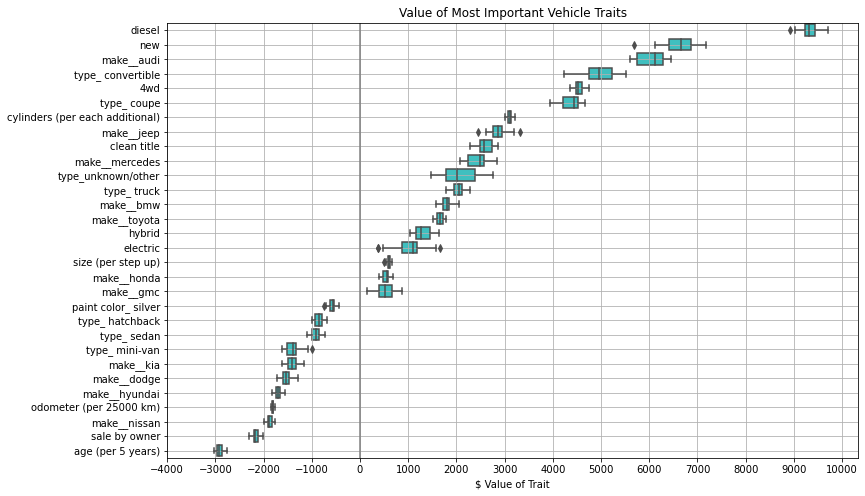
- Trained a linear model (MAE $6,500) to predict a dollar value for important vehicle features (e.g. size, fuel type, manufacturer, odometer, etc.)
- Predictions indicate that diesel vehicles are worth ~$9,000 more than non-diesel vehicles, and that purchasing a vehicle directly from the owner (as apposed to a dealer) can save ~$2,000 off the asking price.
- Exploratory Data Analysis:
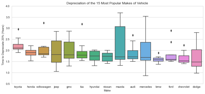
- Found depreciation time constants for the most common vehicle models and manuacturers (e.g. which vehicles ‘hold their value’ the best). Found Toyota, Honda, and Volkswagen depreciate the slowest, while Dodge, Chevrolet, and Ford depreciate the fastest.
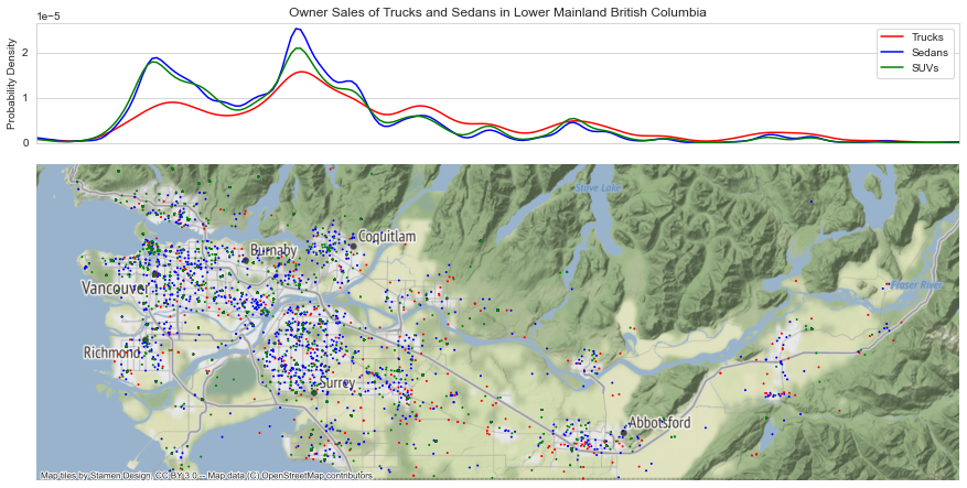
- Produced a geographic distribution of vehicle types in the region (see below). The distribution of trucks was much flatter thoughout the region with smaller peaks around the urban centres, indicating a strong consumer preference for trucks in the suburbs.
- Used interpolation/smoothing to create average contours of price vs odometer reading and age. This gave a benchmark depreciation of $0.20/km driven for the region.
- From price distribution curves, found that sellers tend to price vehicles just under round multiples of $10,000, likely as a psychological pricing strategy.
Code/Resources
Python Version: 3.8.5
Libraries Used: bs4, numpy, pandas, matplotlib, seaborn, scipy, geopandas, contextily, geoplot, sklearn, lightgbm
Craigslist Web Scraping by Riley Predum: https://towardsdatascience.com/web-scraping-craigslist-a-complete-tutorial-c41cea4f4981
Data Science Project Walkthough by Ken Jee: https://github.com/PlayingNumbers/ds_salary_proj#data-science-salary-estimator-project-overview
Linear Coefficient Interpretation: https://scikit-learn.org/stable/auto_examples/inspection/plot_linear_model_coefficient_interpretation.html
1. Web Scraping
I used the tutorial above as a basis to scrape vehicle listings from Craigslist. I needed to expand on the code a fair bit in order to scrape data from each individual vehicle listing page (as apposed to the search page which displays 120 listings at a time). In the end I was able to extract 16 features from each listing:
- body text (the main text of the listing)
- condition (eg. new, salvage)
- drive (front, rear, or 4wd)
- fuel (type of fuel)
- latlong (latitude and longitude associated with the posting)
- location (location associated with the posting, e.g. ‘Vancouver’)
- make (year make and model of the vehicle in a string, e.g. ‘2020 Toyota Corolla’)
- odometer (odometer reading in km)
- paint color
- price (in $ CAD)
- sale type (owner or dealer)
- title status (e.g. clean, rebuilt)
- transmission (manual or automatic)
- type (e.g. sedan, minivan)
- cylinders (number of cylinders in the vehicles engine)
- size (e.g. full-size, compact)
2. Data Cleaning
About 11% of the scaped data was missing values. The columns with missing values were:
- condition: 21.3%
- drive: 24.5%
- odometer: 0.3%
- paint color:29.8%
- type: 30.7%
- cylinders: 37.4%
- size: 57.8%
I opted to fill most of this missing data before going forward. ‘type’, ‘size’, ‘drive’, and ‘cylinders’ were filled with the mode of the data, ‘odometer’ was filled by the mean, and ‘paint color’ and ‘condition’ were replaced with ‘unknown.
Additional cleaning steps were:
- Combine ‘pickup’ and ‘truck’ into one category
- Convert the ‘price’ from a string to a number
- Split the latitude/longitde into distinct numerical columns
- Clean up the location column by taking only the first word of the location with some exceptions
- Split out the year, make and model of the vehicle into separate columns
- Split out the newly created model column into a base model and modifiers (many models have modifiers at the end such as ‘lxt’)
- Create an ‘age’ column by subtracting the current year from the ‘year’ column
- Create new columns based on if the text body contained words I selected as ‘positive’ (e.g. ‘vintage’) or ‘negative’ (e.g. ‘torn’). Also created a column to indicate if the text had few (less than 30) words
3. Exploratory Data Analysis (EDA)
Major graphics and findings from the EDA are below. See the ‘EDA’ notebook for additional details.
3.1 Price Histogram and Density Functions
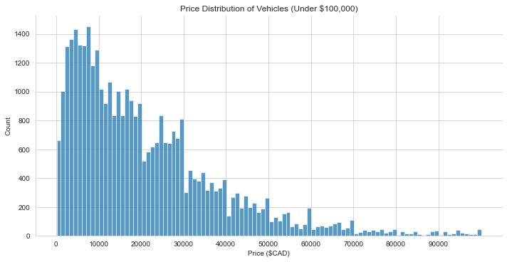
Price distribution for all of the vehichles. The overall distribution is skewed right, with the most common price being between $3,000-$8,000. Note the dips in price at multiples of $10,000. This indicates a psychological pricing strategy (eg. asking $19,000 instead of $20,000 in hopes that the price will seem lower than it actually is).
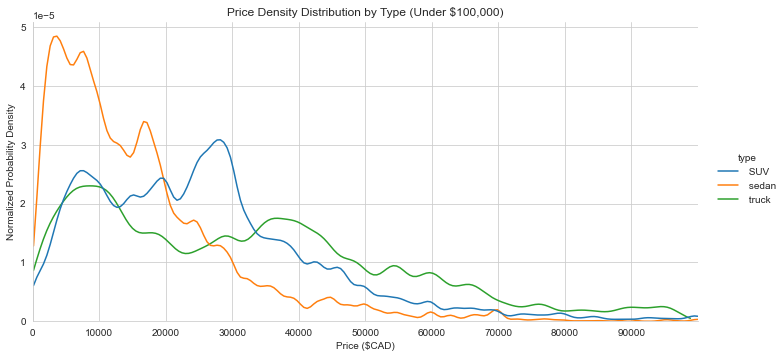
Probability density of price for sedans, SUVs, and Trucks. The curves have been noramlized so the area under each curve is 1. Sedans are the most skewed to the low price end. SUVs and trucks have lower end options (under $10,000) but are also commonly found in the $30,000-$40,000 range. The psychological strategy of pricing just under multiples of $10,000 is more apparent here. This might be a good selling strategy if buyers use the pricing filter their search with a bands at round numbers.
Another interesting feature is the dip in trucks between $15,000 and $30,000, this may indicate there is less turnover in trucks for this price. The mean year and odometer reading for trucks in this price range is 2010 and 170,000km. Perhaps this means people are happy with their trucks in this range, so if you find one it could be a good buy.
3.2 Price Distribution by Odometer and Year
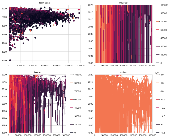
A contourplot of price vs odometer and year can give a birds-eye view of how vehicles depreciate over their lifetime. However generating such as plot is complicated by the noise and sparsity of the pricing data. That is, for a given year and odometer reading, there can be many different prices in the dataset, and the data is not filled in in a nice grid-like fashion. To get around this, the pricing data was first interpolated, then smoothed with a moving average filter.
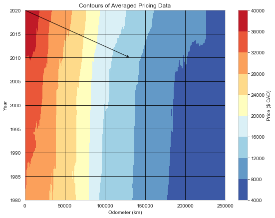
The plots below and to the left show the raw scattered datapoints and three different methods for interpolating into a uniform grid. The ‘nearest’ was chosen and smoothed using a moving average with a window of 30,000km and 3 years. The result is shown on the contour plot below and to the right.
Odometer reading is much more important than year to determine price. According to this data, a newer vehicle would only loose ~20% ($8,000) of its value after 40 years with no driving. On the other hand, the same vehicle driven 50,000km in one year would lose 20-30% of its value.
The arrow on the plot indicates the depreciation for a vehicle driven 13,100 km driven per year (average for British Columbia) for 10 years. This works out to a depreciation rate of $0.20/km.
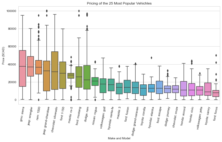
3.3 Pricing of the Most Popular Vehicles
3.4 Depreciation of the Most Popular Vehicles
When buying a car, you are not only interested in the current price, but the future price you might be able to sell it for. Here we will fit a decaying exponential function to individual model of vehicle to quantify the depreciation of that model over time. This will tell us if that model ‘holds its value’. Below is the fit for the Toyota Corolla data.
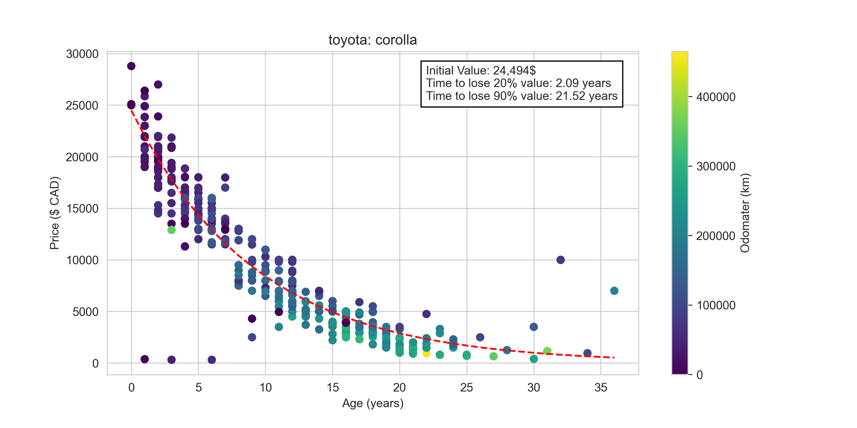
By aggregating the depreciation time constant for the top 10 vehicles under each manufacturer, we can get an idea of which manufacturers hold their value the best. As shown below Toyotas lead the pack with a median time of about 2.1 years for a vehicle to depreciate 20%. Meanwhile a Dodge would only take 1.5 years to depreciate the same fraction. There is still large variability within manufacturers, so it is likely best to determine the depreciation value for the individual model in question when considering a purchase.
3.5 Geographic Distribution of Vehicles
The plot below shows the distribution of sedan, suv, and truck sales by owner in lower mainland BC (where the heighest concentration of data is located). The top probability density curves show the normalized distribution of each vehicle type over longitude. As expected, distinct peaks in both curves occur around Vancouver/Richmond and Surrey where many sales are located.
Note that sedan and SUVs sales are more highly concentrated in the urban centres and truck sales are more evenly distribued. While it might be intuitive that trucks are more likely to be found in the suburbs, it is intersting to note that SUVs are found in high proportion in the city centres alongside sedans.
4 Model Building
4.1 Lasso with Coefficient Interpretation (MAE $6,500)
Lasso is a linear model with an imposed penalty based on the sum of the linear coefficeints. This is useful in dealing with feature co-linearity as some of the coefficents can shrink to zero. The goal for this model was not produce the highest accruacy, but rather produce a set of linear coefficents which can be interpreted as dollar values for a vehicle possessing certain features.
Only the top 15 most popular brans were considered in this analysis. They are (in order of popuularity): Ford, Toyota, Honda, Chevrolet, Mazda, Nissan, Dodge, BMW, Hyundai, Volkswagen, Mercedes, Kia, Jeep, Audi, and GMC.
The model results are shown in the plot below, and can be used to get an idea of the value of the given vehicle traits. Values shown are averages over 5 cross-validation data sets repeated 5 times for a total of 25 models. The error bars show the extent of the data with outliers shown as separate dots. Most traits are ‘yes/no’. The exceptions are cyilnders ($ per cylinder), age ($ per 5 years), odometer ($ per 25,000 km), and size ($ per step up between: sub-compact, compact, mid-size, full-size)
Keep in mind that this linear model is not particularly accurate (MAE $6,500), but it does capture the general trend of the data.
4.2 LightGBM (MAE $2,300)
This tree-based gradient boosting model performed much better than the linear model. Only minor changes to the data were performed before fitting: outliers with a price above $100,000 and odometer above 1,000,000km were droped, and the few rows with missing data were dropped. LightGBM can handle categorical features directly so no encoding was required.
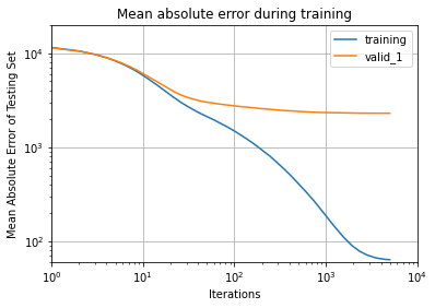
Optimal hyperparameters for the model were found with a cross-validated gridsearch over the entire dataset (sklearn GridSearchCV). Next 20% of the data was held out for validation and training/validation scores were plotted against boosting round iteration. While the training score dropped much lower than the validation score, the validation score at no point started to increase (see below).
With the hyperparameters and number boosting rounds chosen, the model was fit to the entire dataset for productionization.